kangwanying1992gmailcom

The collapse of circulation and the acceleration of upper air superrotation with shortwave optical depth

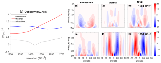
When the atmosphere is more opaque to longwaves than to shortwaves (panel a), the ground temperature is higher than the nearby atmosphere in radiative equilibrium. This jump in temperature causes strong meridional circulation near the surface, especially when the rotation effect is weak (e.g. the tropical regions). This circulation fills the entire troposphere with airs that are almost at rest with the surface, and only above the tropopause, when the stratification is strong enough, the zonal wind U can deviate from 0 following the thermal wind balance.

When the atmosphere is more opaque in shortwaves (panel b), the ground temperature becomes lower than the nearby atmosphere in radiative equilibrium, and therefore meridional circulation becomes suppressed. Zonal wind is only close to zero in the boundary layer, and in the free atmosphere, the zonal wind can vary following the thermal wind balance.

Assuming a semi-gray atmosphere, we analytically solve for the radiative equilibrium temperature profile, based on which we attempt to predict the meridional circulation strength following the “Held-2000 scaling” [1], and the equatorial superrotation.

If you are interested, please see our paper for more details.

Kang, W. and R. Wordsworth 2019, Collapse of the general circulation in shortwave-absorbing atmospheres: an idealized model study, Astrophysical Journal Letter, 885:18, doi: 10.3847/2041-8213/ab4c43

[1] Held, I. M. (2000), The general circulation of the atmosphere, paper presented at 2000 Woods Hole Oceanographic Institute Geophysical Fluid Dynamics Program, Woods Hole Oceanogr. Inst., Woods Hole, Mass.

Regime transition between eddy-driven and moist-driven circulation on High Obliquity Planets

The meridional overturning circulation has two regimes. Under weak insolation and fast rotation, the circulation is dominantly driven by momentum forcing (including friction, eddy momentum transport etc.), and is thermally-indirect in most of the low latitudes (mech anism). Under strong insolation and slow rotation, the circulation is dominantly driven by thermal forcing (including diabatic heating, eddy heat transport etc.), and is thermally-direct.

RL_high_obliquity_S0_Omega3.001 — Panel (a) shows a measure of the contribution of momentum-related processes (blue) and thermal-related processes (red) to the total meridional overturning circulation. Panel (b-g) shows the circulation decomposition for a weak insolation case (top) and a strong insolation case (bottom).

As circulation transforms from a thermally indirect circulation to a thermally direct one, the upper air starts to be filled with low angular momentum air from the extratropics (panel c versus panel b), meanwhile, the low latitudes start to be dominated by downward motion, largely reducing the cloud fraction (panel f versus panel e).

The observables for the regime transition in OBL80-S. (a-c) are for the 10 mb zonal wind, and (d-f) are for the vertically-integrated cloud cover. (a) and (d) show the whole progression of the zonal wind and cloud as insolation increases. While, (b,e) and (c,f) zoom in and show the seasonal cycle at the beginning and the end of the OBL80-S simulation, which corresponds to 1250 W/m2 and 1750 W/m2 insolation. Zero wind speed is denoted with black contours in (a-c).

Reference:

Kang. W. 2019, Regime transition between eddy-driven and moist-driven circulation on High Obliquity Planets, Astrophysical Journal (accepted)

Wetter Stratospheres on High Obliquity Planets

Given that high obliquity aquaplanets tend to be warmer than low obliquity equivalents, we investigate whether the ocean on the warmer high obliquity planets are more vulnerable to strong insolation. The stratospheric water vapor concentration (solid curves) is much higher under high obliquity especially when climate is warm. The stratospheric humidity seems to be better correlated with the maximum surface temperature over the globe throughout the year, rather than the global annual mean surface temperature.

The evolution of upper atmospheric specific humidity and surface temperation with varying insolation. Panel (a) shows the time series of the global mean specific humidity at 10 mb isobar in the solid curves (corresponding to the left axis), and shows that of the global annual mean surface temperature in the dashed curves (corresponding to the right axis), as insolation gradually increases. The high obliquity scenario is in red and the low obliquity is in black. The 1000 ppmv threshold for significant escape is marked by a thin black line. To demonstrate that the insolation change in the transient simulations is slow enough to allow climate to almost reach equilibrium, we repeat the simulation with insolation increased twice as fast. The progression of surface temperature (dots) and upper atmospheric specific humidity (circles) matches the slow-evolving transient experiment reasonably well. Panel (b) is the same as panel (a), except the insolation varies in the opposite direction, decreasing from 1750 W/m2 to 1400 W/m2. As such, the climate remains on the warmer branch rather than the colder branch. Panel (c) scatters the global-mean 10 mb specific humidity against the maximum monthly surface temperature achieved in that year (search among different latitudes and different months). High obliquity in red and low obliquity in black. Extra feedback suppression experiments are also marked in the plot. The red circle denotes a high obliquity experiment forced by fixed annual mean SST, the red “+” sign denotes a similar experiment except that the SST meridional distribution is reversed between the equator and the poles, and the red triangle denotes a high obliquity simulation forced by fixed annual mean insolation. Please refer to the text for more detailed model setups. For reference, the estimated water abundance in the upper atmosphere by 1D model is plot in thin black lines. We, following Kasting et al. 1983, assume moist adiabat from the surface until the temperature falls below the specified stratospheric temperature (marked to the right of each curve).

In addition to the overall warmer climate, the extremely warm period during the polar days, and the misalignment between the cold trap and the spots where water vapor is sent to stratosphere, each is responsible for 1 order of magnitude increase of the stratospheric humidity.

On one hand, a wetter stratosphere makes the ocean more vulnerable to strong insolation, on the other hand, it significantly increases the chance to directly detect surface originated water vapor.

Reference:

Kang. W. 2019, Wetter Stratospheres on High Obliquity Planets, Astrophysical Journal Letter, 877:1, doi: 10.3847/2041-8213/ab1f79

Mechanisms leading to a warmer climate on high obliquity planets

We first find the high obliquity planets to be warmer than their low obliquity equivalents, even when the climate is very warm (1800 W/m2 will blow up the low obliquity experiment), indicating the previously proposed ice-albedo feedback may not be the full story.

Global annual mean surface temperature difference between the high and low obliquity, as insolation gradually increases (solid curve, left axis). Shown on the right axis are the high obliquity (dashed red) and low obliquity (dashed black) mean surface temperature.

Through a series of mechanism-denying experiments, we conclude that the relative warmness stems from the low cloud albedo under high obliquity, which in turn is because the high surface heat capacity makes cloud formation largely lag behind the substellar point migration. As shown below, the high obliquity is warmer than the low obliquity even without ice-albedo feedback, but the temperature difference vanishes or even reverses without cloud radiative effects or without the seasonal variation of insolation.

Annual mean latitudinal surface temperature profile under low obliquity (dark and light blue) and high obliquity (orange and red). Global mean annual mean surface temperature is marked by dashed curves for all cases, and the difference is highlighted by shadings. Shown are for (a) control experiments with all feedbacks on, (b) experiments without ice-albedo feedback, (c) experiments without ice-albedo feedback and without cloud radiation effects, and (d) experiments without ice-albedo feedback and without seasonal cycle (apply annual mean insolation). In (a), there are two equilibrium states for both of the high and low obliquity climate. Dark blue and orange denote the colder equilibrium states, and light blue and red denote the warmer states. In (b,c,d), there is only one equilibrium state, and they are plotted in dark blue and red curves.

Reference:

Kang, W. 2019, Mechanisms leading to a warmer climate on high obliquity planets, Astrophysical Journal Letter, 876:1, doi: 10.3847/2041-8213/ab18a8

Tropical and Extratropical General Circulation with a Meridional Reversed Temperature Gradient as Expected in a High Obliquity Planet

Will the general circulation be just reversed when reversing the meridional temperature gradient?

The simple answer is NO. With a reversed meridional temperature gradient, circulation becomes thermally indirect, shallow, and weak. Explanation is as follows:

Mid-latitude baroclinic eddies become bottom amplified, and this can be explained by the changes of the most unstable mode in the generalized Eady model.

Driven by surface friction (which is required to balance u’v’), the Hadley cell is thermally indirect while the Ferrel cell is thermally direct, in the reverse temperature gradient case, as opposed to the normal gradient case.

Zonal mean meridional circulation streamfunction for the normal case (a,c) and reverse case (b,d). (a,b) are for full eddy simulations and (c,d) are for eddy-free simulations. The streamfunction for the reverse cases (b,d) are in unit 0.2 svp rather than 1 svp as in the normal case. The maxima values are 89 svp, 20 svp, 19 svp and 19 svp respectively for the panel (a,b,c,d).

The eddy-driven Hadley circulation aids to the surface friction driven circulation in the normal case, but cancels it in the reverse case. This partially explained why the reverse case has a weak and shallower circulation compared to the normal case.
The meridional circulation in the reverse case is shallow also because the eddies are bottom amplified in the reverse case and thus there is no strong eddy drag in the upper atmosphere to drive circulation.
The mid-lat Ferrel cell is thermally indirect (direct) in the normal (reverse) case, acting to restore (reduce) the meridional temperature gradient there. This may partially explain why the eddy activity gets much weaker in the reverse case, which then leads to a much weaker meridional circulation.

With seasonal variability (Held Suarez experiment with equilibrium temperature varying with season)…

Annual mean meridional overturning circulation is almost identical to the circulation in the perpetual annual mean simulation.
Solstice Hadley cell is much stronger than the annual mean, and it is driven by eddy heat transport rather than the eddy momentum transport as in the perpetual annual mean simulation.

Reference

Kang, W., M. Cai and E. Tziperman, 2018, Tropical and Extratropical General Circulation with a Meridional Reversed Temperature Gradient as Expected in a High Obliquity Planet, Icarus (und rev.)

MJO-like forcings at different longitudinal locations drive the SSWs to different fates: interaction with the mid-latitude jet zonal asymmetry

The zonal asymmetry of the MJO forcing itself also plays a role. In response to a circumglobal MJO-like forcing, or a longitudinal restricted one located at different locations, the SSWs can be either enhanced or suppressed [5]. Forced by circumglobal MJO-like forcing with increasing amplitude, the SSW first gets enhanced then suppressed as shown in the black solid curve below; this is a result of the competition between the enhancement mechanism and the suppression mechanism.

Fig.7: SSW frequency as a function of the MJO amplitudes for forcings restricted by different longitudinal bands. (Left) uses the wind reversal SSW definition, and (right) identifies SSWs whenever the wind deceleration is stronger than -5m/s/day for 5 days. Copied from [5].

Direct transmission of MJO-excited waves, modification of the stationary pattern in the mid-latitude, and the amplitude of the mid-latitude generated transient waves, all three of them play a role in determining the SSW’s fate. The key process controlling the MJO impact on SSW was found to be the strengthening and weakening of the stationary pattern through the interaction with the MJO forcing. Shown below are the mid-latitude jet response to MJO forcing restricted in B window (where the current MJO forcing located at) and C window (where the future MJO is predicted to expand to). The former (latter) strengthens (weakens) the stationary pattern in the jet, and ends up enhancing (suppressing) the SSWs. Notice that the MJO-excited waves contribute in both cases to enhance SSWs.

Fig.8: (Right panels): Jet structure (250mb U wind)after adding 10K/day MJO forcing in B window and C window. (Left panels): the jet center speed as a function of longitude for different MJO amplitudes in dashed lines; and the difference from the unforced control experiment in solid lines. Copied from [5].

What happens in the transition stage from the unforced background flow to the forced one? We ran 800-ensemble simulations starting from different initial conditions, with the MJO-like forcing turned on at t=0 (initial MJO phase is different from one and another), and closed the momentum budget. The results indicate that the eddy momentum transport, u’v’, drives the climatology response.

Fig.9: (Top panels) show the U250 wind response due to the MJO forcing in (a) window B and (b) window C, with the unforced control U250 profile overlaid as contours. (Bottom panels) show the same U250 response in shading, but show the U wind tendency due to u’v’ eddy momentum transport in contour; the matching indicates the dominant role played by u’v’. Copied from [5].

Reference:

Kang, W. and E. Tziperman, 2018: The MJO-SSW teleconnection: interaction between MJO-forced waves and the mid-latitude jet. Geophysical Research Letter, doi: 10.1029/2018gl077937

Background zonal asymmetry allows MJO to either enhance or suppress the SSWs

Motivation:

Seeing that the MJO-related signal can only propagate to the Arctic in some specific phase (See Fig.1), we anticipated that the zonal asymmetry of either the background state or the forcing itself plays a role and pursued it in Kang and Tziperman 2018 [4].

Findings:

Using idealized circumglobal MJO forcing with k=1 structure, we studied the role played by the background zonal asymmetry. MJO-forced waves can only penetrate the jet in appearance of the background stationary wave pattern. In perfect zonally symmetric experiment (0% below), the transmission rate of the MJO-forced waves decreases to almost zero, consistent with the lackness of MJO-related signal in the Arctic stratosphere (Fig. 5). The transmission rate in the MJO forced experiments (MJO[N]) seem to follow a universal rule as the background changing experiments.

Fig.4: Each solid dot is one background changing experiment (with increasing stationary wave amplitudes in the background flow from 0% to 100%); each empty circle (MJO[N]) denotes one realistic background dry core model forced by MJO forcings with maximum heating rate of N K/day. Shown is the transmission rate of MJO-excited waves through the mid-latitude jet as a function of the maximum U wind convergence at the jet exit region. Copied from [4].

Fig.5: Temperature fluctuation amplitude at the MJO forcing frequency, plotted as a function of pressure and latitude. Without background zonal asymmetry (2dMJO5), the MJO-excited waves cease to propagate before the mid-latitude jet. Copied from [4].

As the transmission of MJO-forced waves being prohibited by the zonally symmetric background flow, the Arctic stratosphere responds in an opposite manner compared to the zonally asymmetric background case: the temperature goes down, the PNJ gets stronger, and the SSW becomes less frequent.

Fig.6: Similar as above, showing the response of temperature, U wind, and SSW time series, but for the response to 5K/day circumglobal MJO-like forcing in a dry core experiment with zonally symmetric background. Copied from [4]

The reason for the suppression of SSWs and the cooling of the Arctic stratosphere is revealed in the U wind response above. The MJO forcing at the Equator works as a wave source, exciting Rossby waves propagating outside the Equator, and in the mean while, transporting momentum to the Equator. As a result, the mid-latitude jet decelerates, the temperature gradient (baroclinicity) falls due to the thermal wind constraint, weakening both the stationary waves and the transient waves which feed on the baroclinicity there.

Reference:

Kang, W. and E. Tziperman, 2018: The Role of Zonal Asymmetry in the Enhancement and Suppression of Sudden Stratospheric Warming Variability by the Madden–Julian Oscillation. J. Climate, 31, 2399–2415, https://doi.org/10.1175/JCLI-D-17-0489.1

Doubling of SSW occurrence due to stronger MJO as expected in a warmer climate.

Motivation:

As the Sudden Stratospheric Warming (SSW) was observed to be led by specific phase of Madden-Julian Oscillation (MJO) [1] , and the MJO was predicted to get stronger under a global warming scenario [2], we started thinking of the behind mechanism of the MJO-SSW teleconnection and the changes in a future warmer climate.

Findings:

We first validated the MJO-SSW teleconnection by showing that the Arctic stratospheric temperature fluctuate with the MJO phase significantly.

Fig.1: Composite of polar cap (65–90N and 10 mb) temperature (K), calculated as an average over all occurrences of a given MJO phase and shown as a function of that MJO phase (horizontal axis) and days since each phase (vertical axis), following Garfinkel et al. (2012a). Results are shown for (a) forced idealized model and (b) WACCM with enhanced entrain- ment and therefore stronger MJO. Copied from [3].

The message deliverer is the large-scale waves excited by the MJO forcing. Shown below is a hovmoller plot of the meridional component of wave activity flux, where the northward propagation of the flux is clear in both WACCM and Idealized dry core model. The signal seems to be halted and noisy around 30N, possibly due to the interaction with the jet there, which turned out to be a key process determining the SSW response (will discuss later).

Fig.2: Hovmoller plot of the meridional component of wave activity flux as a function of latitude and lag time after MJO phase 4 for (left) Idealized dry dynamic core experiment forced by k=1 MJO-like forcing, and (right) WACCM simulation. Copied from [3]

In response to a stronger MJO forcing as expected in a warmer future climate [2], the Arctic stratosphere is warmed by over 4K, the polar night jet is weakened by over 3m/s and the SSW frequency almost doubles, in both a Held-Suarez type idealized model and the Whole Atmospheric Community Climate Model (WACCM).